“Those who do not learn history are doomed to repeat it.”
~George Santayana
It’s important for mankind to learn from the past in order to survive. This notion is true both in personal and professional aspects of live. Every decision we make should be based on some concrete data. This idea seems more relevant for business decisions. So with these things in mind let’s see how to get vital insights from data gathered over time. We will use a dataset and answer some questions using it.
If you know the basics and good to go, skip to the questions.
Before we begin please note that it’s not a traditional tutorial where all basic Pandas functions are explained. Here we will learn functions as and when we need them, with reference to detailed documentation wherever necessary. I will be using a dataset from Kaggle, which has 20 years of computer games history like ratings, platform, editor’s choice etc. You can find it here.
Firsts things first, make sure you have Python (version > 3) on your system along with Pandas (needed to process the dataset), matplotlib (to visualize the data). A quick Google search would fetch you plenty of posts with step by step guide to do that. Now import all the libraries needed :
import pandas as pd
import matplotlib.pyplot as plt
Since the dataset is quite big, to be able to view all columns in the terminal do the following :
pd.set_option('max_columns',None)
pd.options.display.width = None
The above statements remove the upper limit on, maximum number of columns that can be shown and display width . A full list of all supported attributes can be found here. Now that we are all set let’s read the data using Pandas. It’s as easy as this :
data = pd.read_csv("/path_to_file/ign.csv")
This reads the data and stores it in “DataFrame” variable. For those who are new to Pandas, DataFrame is one of the data structures in Pandas which store data in a tabular form or 2D array as we will see later. The other two data structures used in Pandas are Series and Panel explained here. Let’s see what the data looks like :
print(data.iloc[::3][["title","score","score_phrase","genre","platform","editors_choice"]])
DataFrame “iloc” is an attribute that let’s you select rows based on integer index values. For your reference index is the leftmost column in below image. “[::3]” chooses every 3rd row of dataframe. You can view 10th to 50th row (for instance) using “[10:50]” instead. In the next square brackets we pass an array of column labels to show.
This prints below output :
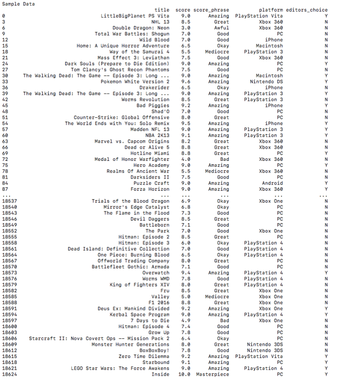
You can remove the columns section and execute to see all the columns. Now let’s try to answer some questions based on this data.
Q1 : What platform has better rated games, PlayStation or Xbox ?
Let’s say you want to a gaming console and you are torn between PS or Xbox. One the important criteria is what games are available for each of them. Thanks to these datasets you don’t have to make a blind decision. Here’s how we are going to do it : group the dataset by “score” column and find the count of PS and Xbox for each group of score. If you look at the “score” column it consists of decimal values which may lead to too many groups and meaning less insight. So first we need to round up the “score” column and store in a new column “score_round”.
data["score_round"] = data["score"].round(0)
Parameter passed to round function tells, up to what decimal places we want to round the decimal number. Please note “round” converts a decimal to nearest number. If decimal is midway (eg. 8.5) it would be rounded to nearest even number (i.e. 8). So 7.5 would be 8 and 8.5 would be 8 too. To visualize our insight in an easy to understand way we must plot the result on bar graph. To do that we store result in a new data frame with 3 columns, ratings, playstation_count, xbox_count.
ratings = sorted(data["score_round"].unique())
data_pf_ratings = pd.DataFrame({"ratings" : ratings})
data_pf_ratings["playstation_count"] = data[data["platform"].str.contains("PlayStation")]["score_round"].value_counts()
data_pf_ratings["xbox_count"] = data[data["platform"].str.contains("Xbox")]["score_round"].value_counts()
First we got all the unique and sorted values of score_round column in an array. Then we created a new data frame “data_pf_ratings” with ratings column only. Next we created new column “playstation_count” count of PS games for each scores (1,2,3 etc). value_counts() groups by and counts the value for each group. Now plot the graph like this :
data_pf_ratings.plot(kind="bar", title="PlayStation vs Xbox",y=["playstation_count","xbox_count"],edgecolor="black",linewidth=1.2)
plt.show()
output :

As you can see PS has a lot more games under 7-10 rating category. Go PlayStation!
Q2 : Is rating of a game dependent on editor’s choice?
This question may seem difficult to answer but thanks to Pandas it’s one of the easiest if you know the concept of “correlation”.
Correlation is a statistical technique that can show whether and how strongly pairs of variables are related.
Pandas has inbuilt function to find correlation :
DataFrame["Col1"].corr(DataFrame["Col2"])
This would return a float value. To give some idea if you use same column in both places in above statement you would get a value of 1.0. So that means a column is completely dependent on itself. But both columns have to be numerical type. The columns that we need to consider in our dataset are “score” and “editors_choice”. So let’s convert editors_choice to numbers and save it in new column “editors_choice_int” :
data.loc[data["editors_choice"] == "Y","editors_choice_int"] = 1
data.loc[data["editors_choice"] == "N","editors_choice_int"] = 0
Now find correlation :
print("Correlation between score and editors_choice")
print(data["score"].corr(data["editors_choice_int"]))
print(data.loc[1:50,["score","editors_choice_int"]].corr())
print(data.corr())
You can use any one of the above ways to get correlation between score and editors_choice columns. Their respective outputs are shown below :
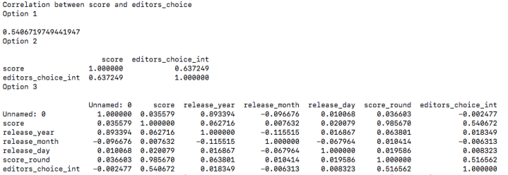
As you can see from 3rd command result all the completely unrelated columns have very less correlation value (except for unnamed 0 & release_year) but score and editors_choice have value of 0.540672. So score dependents on editor’s choice to some extent.
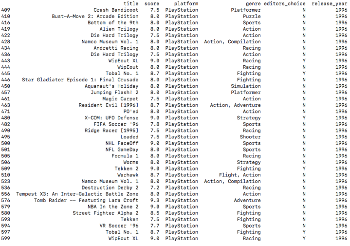
Q3 : Get all games in 1996 by playstation with score > 7?
print(data.loc[(data["platform"].str.contains("PlayStation")) & (data["release_year"] == 1996) & (data["score"] > 7),["title","score","platform","genre","editors_choice","release_year"]])
output :
Q4 : Find the change in game genre (Action/Fight) with year?
Now let’s understand how popular action games have been over the decades. Let’s get a subset of real data which has only action and fight genre games :
data2 = data.loc[(data["genre"].str.contains("Action", case=False, na=False)) | data["genre"].str.contains("Fight", case=False, na=False)]
Now let’s find action/fight game counts for each year :
df_year_to_genre = data2.groupby("release_year")["title"].agg("count").to_frame("count").reset_index()
df_year_to_genre.set_index("release_year").plot(kind="bar", title="Action games per year")
This can also be done using following statement but result won’t be sorted by release_year :
data2["release_year"].value_counts().plot(kind="bar", title="Action games per year")
plt.show()
output :
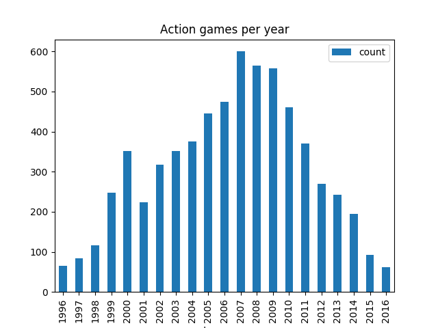
As you can see action game genre has been on the decline since 2010, contrary to what we may believe.
Q5 : What genre gets best ratings (7-10)?
Suppose you have few ideas for developing games under different genres. Which one should you choose. You would obviously want to know what type of games, players like the most. Here’s how :
data_7_10 = data.loc[(data["score"] >= 7)]
dataTemp = data_7_10["genre"].value_counts()
dataTemp[:5].plot(kind="bar", title="Top 5 rated game genres")
plt.show()
It shows top 5 genres like this :
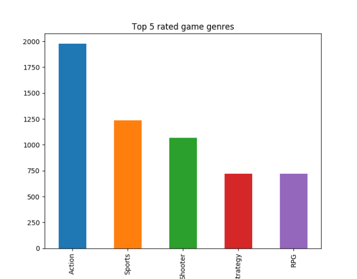
As you can see “Action” is the winner by huge margin.
Q6 : What ratings to Action games usually get?
This question has similar ring to it. It’s just another way to make sure your above decision to delve into action game developement.
print("\nNumber of Action games per rating score")
print(data.loc[(data["genre"].str.contains("Action", case=False, na=False)) | data["genre"].str.contains("Fight", case=False, na=False)].groupby("score_round")["genre"].agg("count"))
“data[“genre”]” returns a series and str is an attribute of series to access contains function.
output :
Number of Action games per rating score

score_round

1.0       12

2.0       94

3.0      148

4.0      514

5.0      509

6.0     1202

7.0     1115

8.0     2022

9.0      710

10.0     139
So most of the action games get ratings of 6-8.
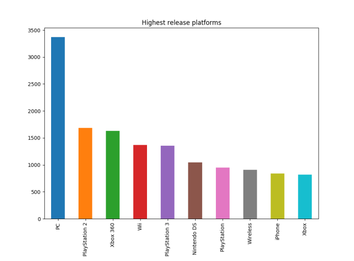
Q6 : What platform do most developers choose?
data_highest_release_pf = data["platform"].value_counts()
data_highest_release_pf[:10].plot(kind="bar", title="Highest release platforms")
plt.show()
output :
Q7 : During what part of year, most games are released?
You went ahead with your idea for action game and developed it with your team. Now comes the time to release it. What is the most suitable time for game release? When do most companies release their games?
data_month_grp = data["release_month"].value_counts().to_frame("count").reset_index()
The above statement finds the count of number of games released in each of year for complete 20 years data and adds it to data frame as new column “count” and resets index of the frame. Why do we need to call reset_index? if we use only
data["release_month"].value_counts().to_frame("count")
it gives a data frame like this :
     count

11   2657

10   2310

9    1707

3    1573

12   1505

6    1483

8    1338

2    1327

4    1264

7    1190

5    1143

1    1128
It gives counts in new column with months of year as index. If we need to use months as a column we should have them in a separate column.
data_month_grp = data["release_month"].value_counts().to_frame("count").reset_index()
This does that. Now dataframe is :
     index  count

0      11   2657

1      10   2310

2       9   1707

3       3   1573

4      12   1505

5       6   1483

6       8   1338

7       2   1327

8       4   1264

9       7   1190

10      5   1143

11      1   1128
data_month_grp = data_month_grp.sort_values(by="index")
data_month_grp.index = ["Jan","Feb","Mar","Apr","May","Jun","Jul","Aug","Sep","Oct","Nov","Dec"]
Now sort data frame by index column and change the inbuilt index to name of months so that on graph we can see month names below each bar to make it intuitive.
data_month_grp.plot(kind="bar", title="Month wise release count")
output :
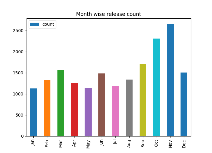
So most of the games are released during year end; mostly during October and November. Is it coincidence or there is actually some reason behind it? We need more data to answer that.
Well then, whatcha waiting for? Find more data and get cracking!
